Logistic Regression is another algorithm of machine learning. It is used for classification type of supervised machine learning. Let’s discuss more about this algorithm and understand it from depth and practical use cases.

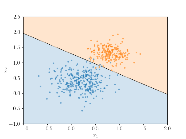
In Logistic Regression, we basically draw a line(or a plane) seperating the classes as binay or multi-class target variable, which means target variable can be of two class as True or False or also can be of mutiple classes as High, Mid or Low. It is predictive model. And also being supervised model, it requires to be fed with training dataset to learn and create a hypothesis function which can predict the outcome(target variable) for new set of input variables.

Let’s first understand the working of Logistic Regression in very naive sense. What this model does is that, It takes every row in consideration and improve the line (or plane) to seperate. To understand it more clearly, let’s assume the line equation is : Ax + By + C = 0

And if a point is actually a negative point(i.e 0) and lies on positive side, we need to bring up the line. And if opposite we need to bring down.

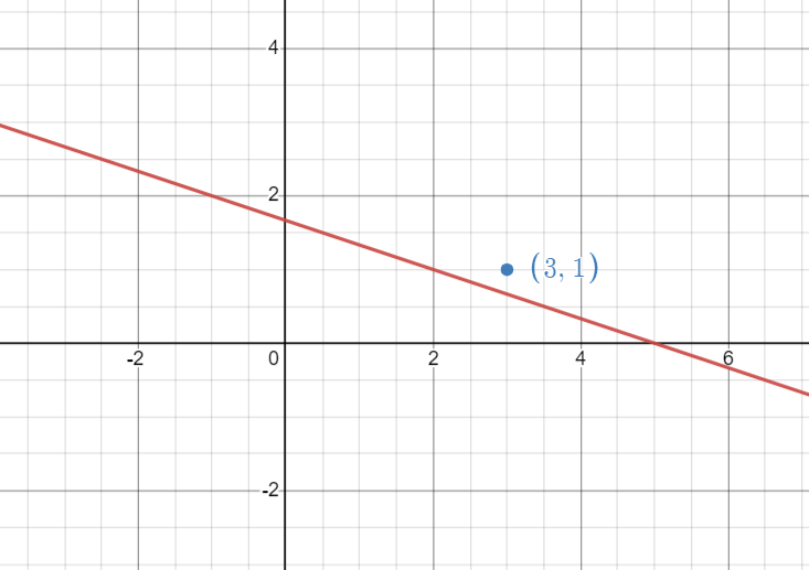
Here if point is negative we need to bring the line (x+3y-5=0) up to keep the point in negative side, to do so we should add the coeffiient of the line with the point. Similary we need to subtract if we had to move the line downward, with the working function,

Wn = Wo + (Yi - Yi(cap))(Xi)

Yi	Yi(cap)	(Yi - Yi(cap))
1	1	0
0	0	0
1	0	1
0	1	-1

This approach is called Perceptron Trick. It has some limitations, as it stops working on improving the line further after it satifies all the training data set. So we have another alternative and better approach to solve this same problem.

Logistic Function :

This alternative to solve the probelm of logistic regression has different working procedure than the former.

In this method, we basically push the correctly classfying line further on correct classification, where the strength of pushing is more when the point is closer to line. Similary, pulls the line on incorrect classification, where the strength (magnitude) of pulling is more when the point is farther and less when closer.

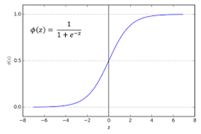
Here also the working function is same as of Perceptron Trick, but the main difference is we use Sigmoid function in Logistic approach, which was step function in former.

Sigmoid function not only gives the decimal value ranging from 0 to 1 despite of 0’s and 1’s. But also it gives the probability of the every line with the points. If the sigmoid function’s value of point is 0.6 it says, there is 60% of point being in positive and 40% of it being negative, being 0.5 point as middle point in sigmoid function.

Unlike step function where value of the crossproduct of coefficient and value of X’s if greater than 0 gives Y as 1 else 0. In Sigmoid, the value of Y is 1 if the result of the sigmoid function when passed the value of cross product gives result greater than or equal to 0.5 else it is 0.

Yi	Yi(cap)	(Yi - Yi(cap))	Remarks
1	0.8	0.2	Little Push(Correct)
0	0.65	-0.65	Strong Pull(Incorrect)
1	0.3	0.7	Strong Pull(Incorrect)
0	0.15	-0.15	Little Push(Correct)

Again, revise this point that when correct and closer larger magnitude push and if incorrect and farther larger magnitude pull.

Implementation

Scikit-learn provides us a predefined LogisticRegression model which we can import easily and use in our code

from sklearn.linearmodel import LogisticRegression
lr = LogisticRegression()
lr.fit(X_train,y_train)
y_pred = lr.predict(X_test)

We can also write our own Logistic Regression Algorithm by following code:

def sigmoid(z):
    return 1/(1+np.exp(-z))

def logistic_function(X,y):
    X = np.insert(X,0,1,axis=1)
    weights = np.ones(X.shape[1])

    for i in range(1000):
        j = np.random.randint(0,X.shape[1])
        y_hat = sigmoid(np.dot(weights[j],X[j]))
        weights = weights - (y[j] - y_hat[j])*X[h]

    return weights[0],weights[1:]

intercept, coeff = logistic_function(X_train,y_train)

Now intercept and coeff can be used to predict the result for new points.

After doing bunch of work we are not able to reach the optimum level of solution, but be patient we are learning it slowly and from scratch so it takes little time to understand. Now a new concept comes into the game called Log-Loss Error.

Minimizing Log Loss Error :

The problem we are here is although we are trying to push the and pull the line to better position we are not doing enough work on loss function. So in this approach our focus will be on to minimizing loss function.

First we calculate the maximum likelihood of any point, that means, we are given with the probability of the points already by sigmoid function now we consider the probability of being positive for positive points and similary being negative for negative points, which can be calculated by 1 - probability of being positive Y(hat).

After that we multiply all the likelihood probability of all the points and try to make it maximum. For eg: If there are two models, one with maximum likehood probability is better.

Now a problem comes, to multiply that many small decimal value will give extremely small value. So, we use log. We know that log(ab) = log(a) + log(b)

Using same rule, multiplication of all the likehoods are seperated to addition using log. We know all the value of likehood probability lies between 0 and 1 and logarithms of number between 0 and 1, all are negative. So to remove negatives, we sum all the negative of the logs. This is called cross entropy.

Cross entropy is the summation of negativelogarithm of likelihood probability. We had to maximize the product of maximum likehood as we study earlier but incase of cross entropy we have to minimize it because log(0.9) < log(0.1) i.e magnitude the log of larger value is less and smaller is larger for numbers between 0 and 1.

So here comes a summary can we write loss function as :

Nope, why not?

Because as we studied earlier, we are taking probability of positive for positive points and negative for negative points, so for negative points it should be log(1-Yi(hat)), which can be formulazied as :

Yi*log(Yi(hat) + (1-Yi)*log(1-Yi(hat))

So in conclusion the loss function can be given by :

This is called Log-loss error and binary cross entropy. Now we need to find coeffient value or (weights) such that error is minimum and there is no any closed form formula to minimize this function like MSE, so we need to use Gradient Descent to minimize the error. Gradient descent to the rescue.

Using Gradient Descent :

Now to write the log-loss error in matrix form. We can say that, Y(hat) = sigma(X*W), where X is the input columns matrix with additional column of ones and W is the matix of weights with one column and rows equal to number of inputs + 1, one for intercept. Similary we hat Y(hat) matrix and Y matrix with equal dimension.

So, Loss Function in Matrix Form:

L = (-1/n)[ Y*log(sigma(X*W)) + (1-Y)*log(1- sigma(X*W)) ]

To minimize L with by changing W, first we initialize W with random numbers and change the W in every iteration to decrease L. Now the fun part is how to change the W, to minimize with every iteration.

We know that in gradient descent we basically use slope and decrement it with old variable(here weights) to get new variable. In this way we move toward least error(L). And plus the learning rate the equation now looks like :

W(new) = W(old) - learning_rate * (dL/dW)

Generally ,if slope is negative the W moves towards positive and if slope is positive the W moves toward negative. So our main task is to find the dL/dW.

Let’s first differentiate first part i.e Y*log(Y(hat)) with respect to W

Then differentiate the second apart i.e (1-Y)*log(1- Y(hat)) with respect to W.

And as a whole the diffrentiation and the working formula will be:

Implementation of GD :

def gd(X,y)
    eta = 0.01
    epoch = 3000
    X = np.insert(X,0,1,axis=1)
    weights = np.ones(X.shape[1])
    for i in range(epoch):
        y_hat = sigma(np.dot(X,weights))
        weights = weights + eta * (np.dot((y - y_hat),X)/X.shape[0])
    return weights[1:],weights[0]

This is how the logistic regression works.

If you have any doubts feel free to raise one. My email [email protected]