You must have heard about the term Gradient Descent in your journey to Data Science. It is one of the most important and widely used algorithm in the field of Machine Learning and as well as Deep Learning.

Basically in simple terms, Gradient Descent is algorithm, an optimization algorithm which repeatedly changes the variables value to have the best solution. To understand more clearly let’s take and example of linear regression. In linear regression we have to find m(slope) and b(intercept). There is a typical way to solve it mathematically by using Ordinary Least Square (OLS) method. But in Gradient Descent approach, we first assume some value of m and b and we iteratively change the value of m and b with the help of training data to get the right pair of m and b finally.

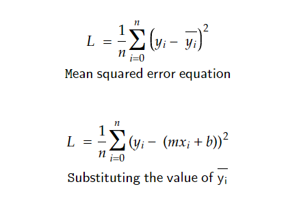
Gradient Descent works on a function which is differentiable at any point and find it’s minimum point. In linear regression, that function is Loss function and our aim to is to minimize it. So we use gradient descent to work on Loss function to minimize it by changing the value of m and b. This is an example for the linear regression but Gradient Descent is not bound to linear regression only.

Gradient Descent is an general algorithm. It is used in Logistic regression, t-SNE algorithm and more on that the whole Deep Learning is based on the gradient descent. That is why this is very important topic. But here in this blog I will use Linear Regression to show it’s implementation.

Working

Gradient Descent is iterative so unlike in OLS, here we use number of iteration to find the value of the m and b. We start with some random value. And those value is given to a function which change the value of m and b repeatedly with a help of function:

m(new) = m(old) - loss_slope_m

b(new) = b(old) - loss_slope_b

Now comes a question, what is two loss_slope here?

Remember we read “loss function” earlier, here the loss_slope is the loss function which is differentiated with respect to both m and b.

loss_slope_m is the diffrentiation of loss function with respect to m whereas the loss_slope_b is the differentiation of loss function with respect to b.

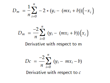
And loss function is the difference of actual Y to the predicted Y by the model. So as our main goal to it is to minimize it. For that we calculate differentiation and equals it with 0 to find the minimum point.

(Now differentiating L w.r to b and L w.r to m)

we get, -2/n _ summation(Y - m _ X - b)

and -2/n _ summation((Y - m _ X - b) * X) as:

There are other 2 things to consider here:

• Learning Rate (denoted by eta)
• Epoch (number of iteration)

Learning rate is used to make the learning procedure of the process more systematical, by adding the term ‘eta’ in the equation as:

m/b(new) = m/b(old) - learning_rate * loss_slope

Implementation

We can create our Gradient Descent Class with the logic understood. It has constructor, fit method and predict method. m and b are initialized whereas learning rate and epoch is passed when object creation. class MyGD:

def __init__(self,lr,epoch):

    self.m = 100 #assumption

    self.b = -100 #assumption

    self.lr = lr

    self.epoch = epoch

def fit(self,X,y):

    n = float(len(X))

    for i in range(self.epoch):

        loss_slope_b = (-2/n) * np.sum(y-self.m*X-self.b)

        loss_slope_m = (-2/n) * np.sum((y - self.m *X - self.b)*(X))

        self.b = self.b - (self.lr * loss_slope_b

        self.m = self.m - (self.lr * loss_sloper_m)

def predict(self,X):

    return (self.m*X)+self.b

As you now understand the some basics of Gradient Descent, let’s head towards little advance concept.

So far what we have learnt is the one type of Gradient Descent and it is Batch Gradient Descent. A question may come, why it is called the “Batch” Gradient Descent.

If you look back in the implementation, we have used entire X data and entire y data in one loop, so it is called Batch GD, and the other types are :

Stochastic Gradient Descent : Unlike Batch one, it updates the m and b value for every single row of X and y pair. So when there is 20 epoch and number of row in X (and y, which are same obviously) is 20. In SGD it runs for 20*20 = 400 loops(or updation of m and b), while in BGD for 20 updation. It is called stochastic because the data are not taken sequentially from 1st row to 2nd and so on. The row are chosen randomly to update the value of m and b.

Advantage of SGD:

• It is suitable for larger data, as the number of epoch can be minimized and it is not necessary to load whole X data in RAM at once for calculation

• It is better for non convex function. Non convex function are the one which has different local minima and global minima. There are times when our model is stops in local minima, in such case SGD can solve the problem.

Probelm in SGD:

• The big variation in the values when it is near the solution can cause problem. Let’s say when it is near the solution but again moves drastically because of bad data in next updation. This can be minimized by learning schedule. The idea is to decrease the learning rate when it is near the solution.

Implementation of SGD:

from sklearn.linear_model import SGDRegressor
reg = SGDRegressor(max_iter=50,learning_rate='constant',eta0=0.01)

where the max_iter is the epoch and learning_rate=’constant’ means the learning_rate is constant for all the iterations, and the value of learning rate is eta0.

Mini Batch GD : It is in between process of Stochastic and Batch GD. It updates after certain number of rows neither like stochastic after every row, nor like batch after all the rows. The number of rows after which the updation is done is called “batch size”.

This was about the Gradient Descent. Learning it lays the foundation to mastering machine learning and also Deep Learning.

If you have any queries, feel free to contact.

My email address : [email protected]