When we start learning about the algorithms in Machine Learning, the first algorithm we encounter with is Linear Regression algorithm(for most of us). It is one of the most used algorithm used for Machine Learning. Most of us have heard about this algo before, not? atleast you heard it when I mentioned it above.

Linear Regression is the algorithm used for Regression based Supervised learning. In regression, we predict the actual value of the output, unlike Classification based which predict the category the output lies on (for eg: True or False, Dog or Cat). As we need a actual value as output for Regression the linear regression algorithm gives us the linear line which tells the property of the data. For example y = 5x + 2. For input value of x as 4, the output value of y will be 22.

Linear Regression(LR) are has different types, mainly Simple LR and Multiple LR. Simple LR is just the example we mentioned above. It has sinlge independent varialbe(input) x for single dependent varialbe(output) y which is actually dependent on x, is in the form of y = mx + b, where m is slope and b is y-intercept, which is defined for a particular line,called Line of Regression and shows two typical property of the line. So when we are doing machine learning with LR, our actual task is to find this line.

What exactly is m and b?

Basically m also called slope is the weightage of x. That means by what parameter the value of x has weight on the value of y, by what amount he value of y depends on value of x.

Whereas the b is the outlier. If the value of x = 0, what will be the value of y.

To understand intercept(b) : For example we have students number of present days as input data and their marks in final exam as output. In such case, if any student is never present in a class, then it is not necessary they have 0 in final exam. So outlers are necessary. Otherwise, it would have y = 0 for x = 0.

Now, we understood what is Simple LR, how to implement in coding. For this, we have a well known machine learning library scikit-learn which has all the necessary machine learning algorithm and also other facility.

One of the facilites is to split our input(x) and output(y) as train and test data. It split such that they training set and test set are independent to each other. Otherwise the overfitting will occur.

from sklearn.model_selection import train_test_split
X_train,X_test,y_train,y_test = train_test_split(X,y,test-size=0.2)

After done spliting we can import linear regression to train the algorithm for creating the line to represent our data in the form of y = mx + b.

from sklearn.linear_model import LinearRegression
lr = LinearRegression()
lr.fit(X_train,y_train)

We can also print the value of m and b for our line by following line of code

m = lr.coef_
b = lr.intercept_

What exactly is done by scikit-learn under the hood?

Basically to produce the a line of equation y = mx + b, the scikit-learn runs some logic, which is just the mathematics behind the Linear Regression. If we learn this logic, we can create our own .

To find the value of m and b:

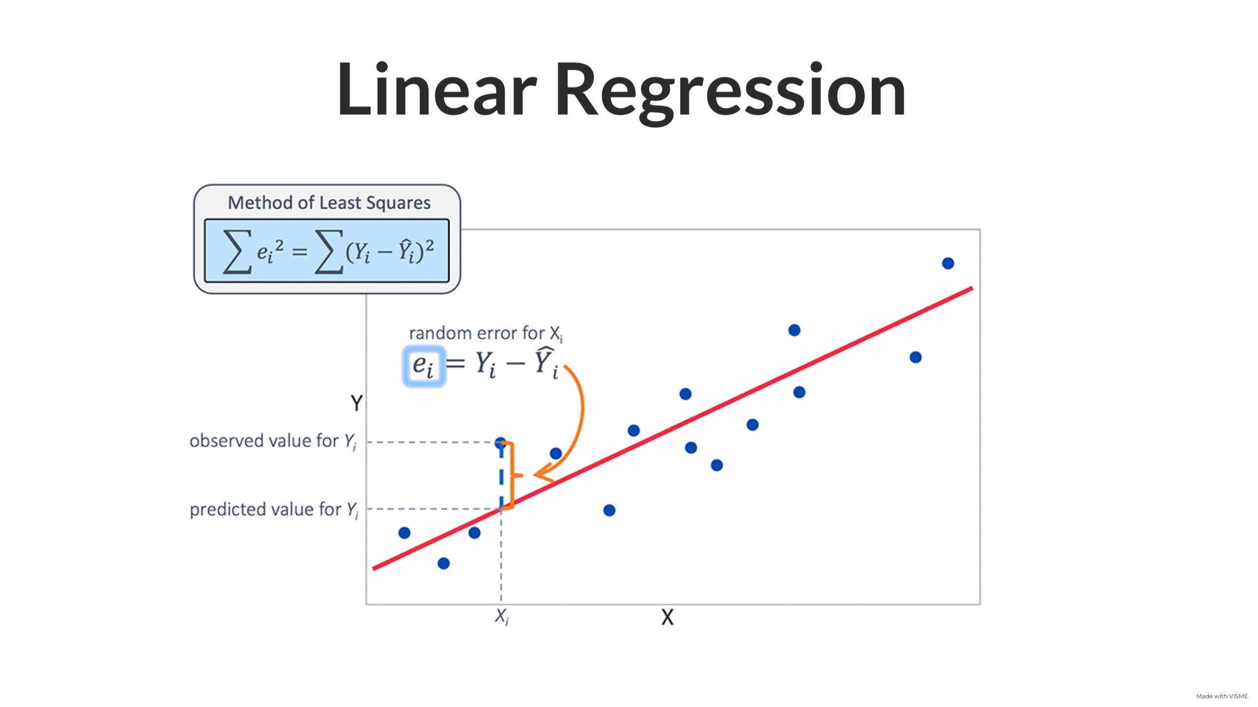
Always keep in minde, Linear regression is error correction method.

Let’s assume the value of Y at Xi is Yi as per the linear regression’s line but actually it was Y(cap) as per the the data. So here the error is Yi-Y(cap), which is squared to remove the negative element(because it could be up or down, which Yi-Y(cap) could be positive or negative).

Y(cap) is the actual location of point so it can be written as: Y(cap) = mXi+b

So E(m,b) = (summation from i to n) (Yi-mXi-b)^2 Now our goal is to minimize this error(E).

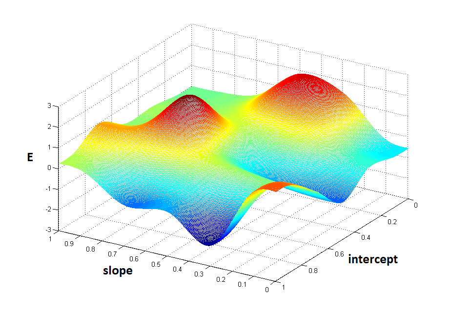
We know that slope is 0 at the minimum point and the slope is given by the first order differentiation of the E. First, we differentiate E with respect to ‘m’ and differentiate it with respect to ‘b’.

<differentiation of E = Yi - mXi - b w.r to b>

So the value of b = Y(bar) - mX(bar) And, now using b in E to differentiate w.r to m:

<differentiation of E = Yi - mXi - b w.r to m>

So, the value of m becomes = (X-Xi)(Y-Yi)/(X-Xi)^2 Now, when we know the logic behind calculation of m and b. We can implement this in code:

class MyLR:
	def __init__(self):
		self.m = None
		self.b = None
	def fit(self,X_train,y_train):
		num = 0
		den = 0
		X_mean = X_train.mean()
		y_mean = y_train.mean()
		for i in range(X_train.shape[0]):
			num = num +  (X_train[i] - X_mean)(y_train[i]-y_mean)
			den = den +  (X_train[i]-X_mean)*X_train[i]-X_mean)
		self.m = num/den
		self.b = y_mean - m*(X_mean)
	def predict(self,X_test):
		return (self.m*X_test)-self.b

Similarly we have multiple linear regression where the equation is in form of

Y = b0 + b1X1 + b2X2 + ..... bmXm

where m in the number of features in input. And a plane is used instead of line in the (m+1)D space.

The above equation can be represented as : Y = XB, where B is betas(b0,b1,…..)

So similar to simple linear regression, the error in each point is given by Yi-Y(cap). And the total error is given by E = e^T.e and replacing Y(cap) by XB.

E = (Y^T -Y^TXB - (XB)^TY + (XB)^TXB

When differentiating it with B, and equals to 0 for minimum point, we get:

B = (X^TX)^-1.X^T.Y

Now, when we implement it with code to make your own Multiple Linear Regression algorithm:

class MyLR:
	def __init__(self):
		self.coef_
		self.intercept_

	def fit(self,X_train,y_train):
		X_train = np.insert(X_train,0,1,axis=1)

		betas = np.linalg.inv(np.dot(X_train.T,X_Train)).dot(X_train.T).dot(y_train)
		self.intercept_ = betas[0]
		self.coef_ = betas[1:]

	def predict(self,X_test):
		y_pred = np.dot(X_test,self.coef_) + self.intercept_
		return y_pred

This is the general approach for Linear Regression in closed form, OLS method. Linear Regression can be done with Gradient Descent Technique also, more on that on the next blog.

I hope you understood something about Linear Regression from this article. Feel free to raise queries by contacting me. I will to try to solve your confusions.